Product Variety and Commonality

Marketing Drivers of Product Variety

Estimate the inventory benefits of using
part commonality to achieve
product variety

Skip the intro, take me to the Calculator

Marketing Drivers of Product Variety

In many industries, customers demand highly customized products to meet their individualized needs. Companies often respond by increasing the product variety — or the number of variety dimensions and corresponding options — made available to customers.

For example, a bicycle company may offer mountain bikes, road bikes, and racing bikes. Within each class of bikes, it may offer options along various dimensions such as color (red, blue, silver, etc.), geometry (men’s, woman’s, front suspension, full suspension, etc.), size (15″, 16″ 17″, 18″, etc.), materials (steel, aluminum, titanium, carbon fiber, etc.), component performance (H, M, L, etc.), and so on.

It doesn’t take long for the potential complexity to get mind-boggling. Consider even the variety offered by our hypothetical bicycle company. If all combinations are permissible, there would be 1,728 possible end items (3 x 3 x 4 x 4 x 4 x 3).

Design Drivers of Product Variety

The variety that is driven by the dimensions valued by customers is clearly intended to increase revenue and market share. Variety can also be the result of efforts to decrease the material costs or increase the technical performance of parts and sub-systems. The performance that is required of a component depends on the product that it is eventually assembled into. For example, handle bars on larger bikes will likely face more stress (heavier riders) than handle bars on smaller bikes. Designers could save material costs by specifying thinner bars on smaller bikes. Inevitably, however, the result will be another dimension of variety. People come in all shapes and sizes, so some short and heavy riders will want thicker bars for strength and some tall and thin riders will want thinner bars for weight savings.

Complexity Costs

If the benefits of variety are higher revenues, lower material costs, and better technical performance, what are the costs? Product variety often increases the cost of things such as design, tooling, information systems, manufacturing, inventory, and after-sales support.

Commonality as a Strategy

Commonality is one approach adopted by many manufacturers to keep these “costs of complexity” under control. With commonality, the same version of a part or sub-system (we will refer to either as a “component”) is shared across multiple products. To avoid damaging perceived differentiation, designers often standardize the components that customers don’t care that much about. For example, bicycle companies often standardize components such as handle bars, frame tubes, brake- and shift-cables, tires, etc. These common components are engineered to meet the most stringent requirements and then “substituted downwards.” In other words, some products will have components that are “better than they need to be.” In other words, “higher cost than they need to be.”

Inventory Benefits of Commonality

So, what are the inventory benefits of commonality? The main benefit is reduced safety stock through lower forecast error. Intuitively, people understand that it is easier to forecast an aggregate quantity (e.g. all bikes sold in June) than individual items (e.g. the number of blue, front-suspension, 18″, steel mountain bikes with high-end component sets that are sold in June). If every bike shares a standard handle bar, then it will be easier to forecast consumption of handle bars, and handle bar inventory costs will be lower. The reduction of forecast errors through aggregation of demand is often called “risk pooling.”

The calculator on this page will help you understand the inventory benefits of commonality under three situations.

Take me to the Calculator

Situation 1: The common component is used across all products, also known as a universal component. Example: All bikes use the same handle bar.

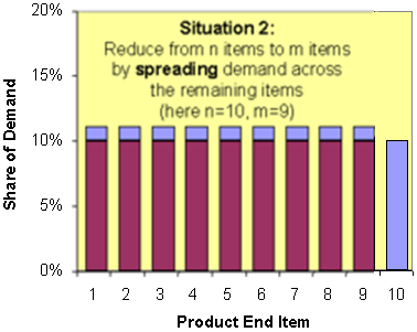
Situation 2: The common component allows you to spread the demand of one or more eliminated products across the remaining products. Example: Offer frame sizes that are 2″ apart, so riders pick the closest size and then adjust the seat height.

Situation 3: The common component allows you to consolidate the demand of two or more products together. Example: Make the geometry for the men’s frame the same as that of the front suspension frame.

See below for a more detailed description of all the parameters used in this calculator. Note that because of the assumptions made, this calculator generally provides an upper-bound on inventory savings achieved through risk-pooling.

To use the calculator, simply change one or more of the blue numbers and then click the Calculate button.

Number of End Items
Item count before (n)		number
Item count after (m)		number
Inventory Carrying Costs
Annual holding cost (h)		(%)
Inventory cost (c)		($/unit)
Safety Stock
Target service level (SL)	99.9% 99% 98% 97% 95% 90% 85% 70% 50%
Forecast error (fe)		(%)
Lead time (L)		(weeks)
Review period (R)		(weeks)
What is the cost of safety stock?
Inventory cost		($/unit/WOS)
Safety stock (SS)		(WOS)
Safety stock cost		($/unit)
What are the potential savings in safety stock? Situation 1: If you could design a universal item, it might be worth spending as much as $/unit more in material costs. Situation 2: In going from from items to items by spreading demand across the remaining items, it might be worth spending as much as$/unit more in material costs. Situation 3: In going from from items to items by consolidating demand onto one particular item, it might be worth spending as much as $/unit more in material costs.

To Introduction Reload Page

Note: These calculators were created to facilitate rapid analysis of DFSC decisions. Although these calculators make simplifying assumptions, they have proved useful in practice. For complex trade-offs of additional cost factors or for especially important decisions, you may want to perform a more detailed analysis.

Inventory Parameters

• Demand: Mean demand or consumption at an inventory stockpile (units/week). In this calculator, we assume demand of all items is the same.
• Forecast error (fe): Standard deviation of the difference between forecasted and actual customer orders, divided by the mean demand. This ratio is sometimes also called coefficient of variation (CoV). In this calculator, we assume forecast error for all items is the same. Lead time (L): Mean lead time to replenish product into an inventory stockpile (weeks). In this calculator, we assume that lead time for all items is the same.
• Lead time uncertainty (lu): Standard deviation of replenishment lead time divided by the mean lead time. In this calculator, we assume no lead time uncertainty.
• Target service level (SL): The desired percentage of demand periods where there are no stock-outs. It is sometimes called availability rate. Depending on the target service level, safety stock is scaled up or down by a factor “k.” In this calculator, we assume that target service level for all items is the same.
• Review period (R): The period of time in-between physical review of inventory stockpiles (weeks). It is assumed that replenishment orders are placed after each inventory review. For continuous review systems, R is zero. In this calculator, we assume review period for all items is the same.
• Inventory cost (c): The current cost of the inventory, including material costs and any incremental value-add ($/unit).
• Annual inventory holding cost (h): Expressed as a percentage of inventory cost, the annual inventory holding cost typically includes financing, storage, devaluation, and scrap.
• Inventory weeks of supply: Inventory units divided by the mean weekly demand (WOS).

---